How to Freeze Panes in Excel: Keep Rows and Columns Visible While Scrolling

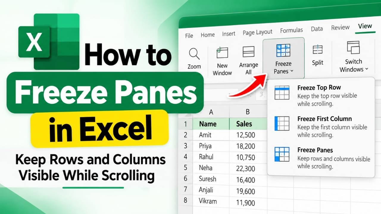
When an Excel worksheet contains many rows or columns, it can become difficult to remember which data belongs to which heading. Freeze Panes solves this problem by keeping selected rows or columns visible while you scroll through the rest of the worksheet.

In Excel, you can freeze the top row, the first column, or multiple rows and columns at the same time. The feature only changes the way the worksheet appears on screen; it does not alter your actual data.

Also read: How to Recall an Email in Outlook: Step-by-Step Guide

How to Freeze the Top Row in Excel

If your worksheet has column headings in the first row, freezing the top row can make large spreadsheets easier to read.

Follow these steps:

1. Open your Excel worksheet.
2. Go to the View tab.
3. Click Freeze Panes.
4. Select Freeze Top Row.

A line will appear below the first row. Now, when you scroll down, the first row will remain visible.

This is particularly useful for spreadsheets where the first row contains headings such as Name, Date, Amount, Status, or ID.

How to Freeze the First Column in Excel

You can also keep the first column visible while moving horizontally across a worksheet.

1. Open the worksheet.
2. Select the View tab.
3. Click Freeze Panes.
4. Choose Freeze First Column.

Column A will remain visible when you scroll to the right.

This can be useful when the first column contains information such as employee names, product names, customer IDs, or other identifiers.

How to Freeze Multiple Rows or Columns

Excel also lets you freeze several rows and columns together.

The important thing to understand is that Excel freezes the rows above and columns to the left of the cell you select.

For example:

• Select A4 to keep rows 1–3 visible.
• Select B2 to keep row 1 and column A visible.
• Select C4 to keep rows 1–3 and columns A–B visible.

Steps to freeze multiple rows or columns

1. Click the cell immediately below and to the right of the rows and columns you want to keep visible.
2. Go to View.
3. Select Freeze Panes.
4. Click Freeze Panes again from the menu.

Excel will keep the selected upper rows and left-side columns visible while you scroll.

Example

Suppose your worksheet has three heading rows and you also want column A to remain visible.

Select B4 because:

• Rows 1–3 are above B4.
• Column A is to the left of B4.

Then choose View > Freeze Panes > Freeze Panes.

How to Unfreeze Panes in Excel

If you no longer want rows or columns to remain fixed:

1. Open the View tab.
2. Click Freeze Panes.
3. Select Unfreeze Panes.

Once panes are frozen, Excel changes the relevant menu option to Unfreeze Panes.

How to Freeze Panes in Excel for Mac and the Web

The Freeze Panes feature is also available in other versions of Excel.

Excel for Mac

Use the View tab and select Freeze Panes. From there, you can choose the appropriate freezing option.

Excel for the Web

Open the worksheet and go to View > Freeze Panes. Select the rows, columns, or panes you want to keep visible.

Excel on iPhone, iPad, or Android

In the mobile version of Excel, open View, select Freeze Panes, and choose the available option for the top row, first column, or panes.

The exact interface can vary slightly depending on the Excel version and device.

Why Is Freeze Panes Grayed Out in Excel?

Sometimes the Freeze Panes option may not work as expected. A few common reasons include:

You are currently editing a cell

If you are typing inside a cell, finish the edit by pressing Enter or Esc, then try Freeze Panes again.

Excel is in Page Layout view

Switch back to Normal view from the View tab and try again.

The worksheet is protected

A protected worksheet may restrict certain changes. Check the Review tab to see whether the sheet is protected and whether you have permission to make the required changes.

Does Freezing Rows Affect Printing?

No. Freeze Panes is primarily a screen-view feature.

If you freeze the first row, it will remain visible while you scroll through the worksheet on your screen. It does not automatically make that row appear at the top of every printed page.

If you need column headings to repeat on every printed page, you need to configure Excel’s print settings separately.

Can You Freeze a Row in the Middle of an Excel Sheet?

Not by itself.

Freeze Panes works from the top of the worksheet and the left side. For example, you cannot simply tell Excel to keep row 20 visible while rows 1–19 scroll away.

If you need to view two different areas of a worksheet at the same time, Excel’s Split feature may be more appropriate. You can find it under View > Split.

Freeze Panes vs. Split in Excel

These two features serve different purposes:

Feature	What it does
Freeze Panes	Keeps selected top rows and left columns visible while scrolling
Split	Divides the worksheet into separate scrollable areas

For a large data table with headings, Freeze Panes is generally the feature you need.

Frequently Asked Questions

Also read: How to Clear Cache on Android: A Simple Step-by-Step Guide

Conclusion

Freeze Panes in Excel is useful when working with large worksheets because it keeps important headings or identifiers visible while you scroll. You can freeze the top row, first column, or a combination of rows and columns by selecting the appropriate cell before using View > Freeze Panes.

If you only need to keep column headings visible, Freeze Top Row is usually enough. For more complex worksheets, selecting the correct cell before choosing Freeze Panes lets you control exactly which rows and columns stay on screen.