How to Use VLOOKUP in Excel: A Practical Guide With Examples

If you need to find a value in an Excel table and return related information from the same row, VLOOKUP is one of the most useful functions to know. It can help you find a product price from an ID, retrieve an employee department, match customer information, or assign a grade based on a score.

The basic formula is:

=VLOOKUP(lookup_value, table_array, col_index_num, FALSE)

For example, =VLOOKUP(E2,A2:C20,3,FALSE) searches for the value in E2 in the first column of A2:C20 and returns the corresponding value from the third column.

This guide explains how VLOOKUP works, how to create formulas, how to copy them correctly, how to troubleshoot common errors, and when XLOOKUP or INDEX/MATCH may be a better choice.

Also read: How to Unhide All Rows in Excel: Step-by-Step Guide for Windows, Mac and Web

What Is VLOOKUP in Excel?

VLOOKUP stands for Vertical Lookup. It searches for a value down the first column of a selected range and returns information from another column on the same row.

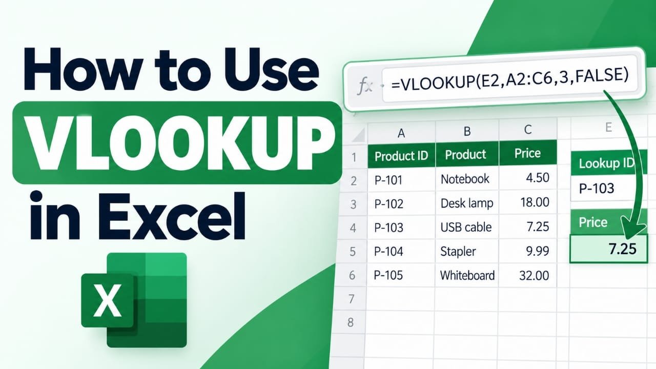
For example, suppose you have this table:

Product ID	Product	Price
P-101	Notebook	4.50
P-102	Desk lamp	18.00
P-103	USB cable	7.25
P-104	Stapler	9.99
P-105	Whiteboard	32.00

If cell E2 contains P-103, you can use VLOOKUP to find the product’s price:

=VLOOKUP(E2,A2:C6,3,FALSE)

Excel searches for P-103 in column A and returns 7.25 from column C.

VLOOKUP Syntax Explained

The complete VLOOKUP syntax is:

=VLOOKUP(lookup_value, table_array, col_index_num, [range_lookup])

Each argument has a specific job.

1. lookup_value

This is the value you want Excel to find.

It could be:

• A cell reference such as E2
• A number
• Text such as "P-103"

2. table_array

This is the range containing your lookup data.

The first column of this range must contain the value you’re searching for. The information you want VLOOKUP to return must be somewhere to the right.

For example:

A2:C6

means VLOOKUP searches column A and can return information from columns B or C.

3. col_index_num

This tells Excel which column of the selected range contains the result.

The count starts at the left edge of the selected range, not from worksheet column A.

For A2:C6:

• Column A = 1
• Column B = 2
• Column C = 3

So this formula returns the product name:

=VLOOKUP(E2,A2:C6,2,FALSE)

While this one returns the price:

=VLOOKUP(E2,A2:C6,3,FALSE)

4. range_lookup

This controls how Excel searches for a match.

Use:

• FALSE or 0 for an exact match
• TRUE or 1 for an approximate match

For most ordinary lookups, FALSE is the safer choice.

If you leave this argument out, VLOOKUP uses approximate matching by default. That can produce unexpected results when the first column isn’t arranged correctly.

How to Create a VLOOKUP Formula

Here’s a simple way to create one from scratch.

1. Click the cell where you want the result.
2. Type =VLOOKUP(.
3. Select the cell containing the value you want to find.
4. Enter a comma.
5. Select the table containing your data.
6. Enter another comma.
7. Enter the number of the column containing the answer.
8. Enter another comma.
9. Type FALSE.
10. Close the parenthesis and press Enter.

For example:

=VLOOKUP(E2,A2:C6,3,FALSE)

If E2 contains P-103, the result is 7.25.

You can then change E2 to another product ID, and the returned value updates automatically.

A Simple VLOOKUP Example

Suppose your worksheet contains:

Product ID	Product	Price
P-101	Notebook	4.50
P-102	Desk lamp	18.00
P-103	USB cable	7.25
P-104	Stapler	9.99
P-105	Whiteboard	32.00

Enter P-103 in E2.

Then enter:

=VLOOKUP(E2,A2:C6,3,FALSE)

The formula returns:

7.25

If you change the column number from 3 to 2:

=VLOOKUP(E2,A2:C6,2,FALSE)

the result becomes:

USB cable

This is because the second column of the selected range contains the product name.

How to Copy VLOOKUP Down a Column

A common problem occurs when you copy a VLOOKUP formula to multiple rows.

Suppose the original formula is:

=VLOOKUP(E2,A2:C6,3,FALSE)

When you drag it down, Excel may change the table range to A3:C7, then A4:C8, and so on. Eventually, the formula may stop looking at the correct data.

The solution is to make the table range absolute.

Use:

=VLOOKUP(E2,$A$2:$C$6,3,FALSE)

The $ signs keep the table range fixed when the formula is copied.

You can add these references manually or select the range in the formula and press F4 in Excel.

When you drag the formula down:

• E2 becomes E3, E4, E5, etc.
• $A$2:$C$6 stays unchanged.

This is especially important when you’re applying the same lookup to a long list.

Using VLOOKUP With Approximate Match

VLOOKUP isn’t limited to exact matches. An approximate match is useful when your table contains ranges or thresholds.

Typical examples include:

• Grade boundaries
• Tax brackets
• Commission levels
• Shipping charges
• Discount tiers

Consider this grading table:

Minimum Score	Grade
0	F
60	D
70	C
80	B
90	A

The first column represents the minimum score required for each grade.

If D2 contains 84, use:

=VLOOKUP(D2,$A$2:$B$6,2,TRUE)

The result is B.

Why? Excel finds the largest number in the first column that is less than or equal to 84. In this case, that number is 80.

Important rule for approximate VLOOKUP

The first column must be sorted from smallest to largest.

If it isn’t sorted correctly, an approximate lookup can return an incorrect result.

For ordinary ID, name, or product searches, use FALSE instead.

Using Wildcards With VLOOKUP

VLOOKUP can also use wildcards for text searches when you use an exact-match lookup.

The main wildcard characters are:

• * — represents any number of characters
• ? — represents one character
• ~ — treats * or ? as an actual character

For example, with a product list, this formula:

=VLOOKUP("Desk*",B2:C6,2,FALSE)

can find a product beginning with “Desk”.

A wildcard lookup returns the first matching result, so the search pattern should be specific enough when multiple rows could match.

How to Use VLOOKUP on Another Worksheet

Your lookup table doesn’t need to be on the same worksheet as the formula.

For example, suppose your lookup table is on a sheet named Prices.

You can use:

=VLOOKUP(A2,Prices!$A$2:$C$6,3,FALSE)

Here:

• A2 is the value being searched for.
• Prices!$A$2:$C$6 is the table on the Prices sheet.
• 3 tells Excel to return the third column.
• FALSE requires an exact match.

If the worksheet name contains spaces, Excel uses single quotation marks.

For example:

=VLOOKUP(A2,'Client Details'!$A$2:$C$6,3,FALSE)

Using VLOOKUP With Another Workbook

VLOOKUP can also retrieve information from another Excel file.

A typical process is:

1. Open both workbooks.
2. Start the VLOOKUP formula in the workbook where you want the result.
3. Select the lookup value.
4. Switch to the workbook containing the source data.
5. Select the lookup table.
6. Finish the remaining arguments.
7. Press Enter.

Excel creates an external workbook reference automatically.

If the source workbook is later moved, renamed, or its location changes, the external reference may need to be updated.

For that reason, external VLOOKUP links should be managed carefully when files are shared between computers or folders.

Common VLOOKUP Errors and How to Fix Them

VLOOKUP errors are usually caused by a small issue with the formula or source data.

#N/A

This usually means Excel couldn’t find the requested value with an exact match.

Check:

• Is the lookup value actually present?
• Is the lookup column the first column of the selected range?
• Are there extra spaces?
• Are the two values stored using the same data type?
• Does the table range include the required row?

#REF!

This happens when the column number is larger than the number of columns in the selected range.

For example:

=VLOOKUP(E2,A2:C6,4,FALSE)

is invalid because A2:C6 contains only three columns.

#VALUE!

A column index below 1 can cause this error.

Check the col_index_num argument.

#NAME?

Check the function name and any text values.

For example, text should be enclosed in quotation marks:

=VLOOKUP("P-103",A2:C6,3,FALSE)

not:

=VLOOKUP(P-103,A2:C6,3,FALSE)

#SPILL!

This can occur when the lookup value is supplied as an entire column rather than a single value.

For example:

=VLOOKUP(A:A,A:C,2,FALSE)

may cause a spill-related problem. Use an individual cell reference where appropriate.

Why VLOOKUP Returns the Wrong Result

A formula can be syntactically correct and still return the wrong value.

One common reason is leaving out the final argument:

=VLOOKUP(E2,A2:C6,3)

Because the match type is omitted, Excel uses approximate matching.

If you need an exact match, write:

=VLOOKUP(E2,A2:C6,3,FALSE)

Another common problem is failing to lock the table range before copying the formula.

Use:

=VLOOKUP(E2,$A$2:$C$6,3,FALSE)

rather than:

=VLOOKUP(E2,A2:C6,3,FALSE)

What to Do When VLOOKUP Shows #N/A

If you can see the value in the table but VLOOKUP still returns #N/A, work through these checks:

1. Check the first column
   Make sure the lookup value is in the leftmost column of the selected range.
2. Check the range
   Make sure the range includes the row containing the value.
3. Look for unwanted spaces
   An extra space can prevent an exact match.
4. Check data types
   A number stored as text isn’t always treated the same as a real number.
5. Check the copied formula
   Make sure the table range hasn’t moved.

If unwanted spaces are the problem, TRIM can help:

=VLOOKUP(TRIM(E2),$A$2:$C$6,3,FALSE)

You can also display a friendlier message when a value doesn’t exist:

=IFNA(VLOOKUP(E2,$A$2:$C$6,3,FALSE),"Not found")

IFNA specifically handles the #N/A result. It doesn’t eliminate other errors, so it’s better to fix the underlying formula first.

VLOOKUP vs XLOOKUP vs INDEX and MATCH

VLOOKUP isn’t the only way to find related information in Excel.

Function	Can look left?	Match behavior	Column number required?
VLOOKUP	No	Approximate by default	Yes
XLOOKUP	Yes	Exact by default	No
INDEX + MATCH	Yes	Controlled by MATCH	No

For example, to find the price of P-103, VLOOKUP can use:

=VLOOKUP(E2,A2:C6,3,FALSE)

XLOOKUP can use:

=XLOOKUP(E2,A2:A6,C2:C6,"Not found")

INDEX and MATCH can use:

=INDEX(C2:C6,MATCH(E2,A2:A6,0))

XLOOKUP is available in newer versions of Excel, while VLOOKUP is useful when working with older Excel versions that don’t support XLOOKUP.

Another advantage of XLOOKUP is that the lookup and return ranges are specified separately. You don’t have to count columns within a table.

Which one should you use?

Use VLOOKUP when:

• You need compatibility with older Excel versions.
• The lookup column is to the left of the result.
• You want a familiar, straightforward formula.

Use XLOOKUP when:

• Your Excel version supports it.
• You want to look in either direction.
• You want a built-in result for missing values.
• You prefer separate lookup and return ranges.

Use INDEX and MATCH when:

• You need a flexible lookup approach.
• The lookup column isn’t the leftmost column.
• You need compatibility with older Excel versions.

Frequently Asked Questions

Also read: How to Make a Pie Chart in Excel

Conclusion

VLOOKUP is useful when you need to match a value in one column and retrieve related information from another column. For most straightforward searches, use an exact-match formula with FALSE, and lock the table range with $ signs when copying the formula.

Once you understand the four arguments—lookup value, table range, column number, and match type—you can use VLOOKUP for everything from simple product searches to range-based lookups.

For newer Excel versions, XLOOKUP is another strong option, particularly when you need to search in either direction or handle missing results more conveniently.