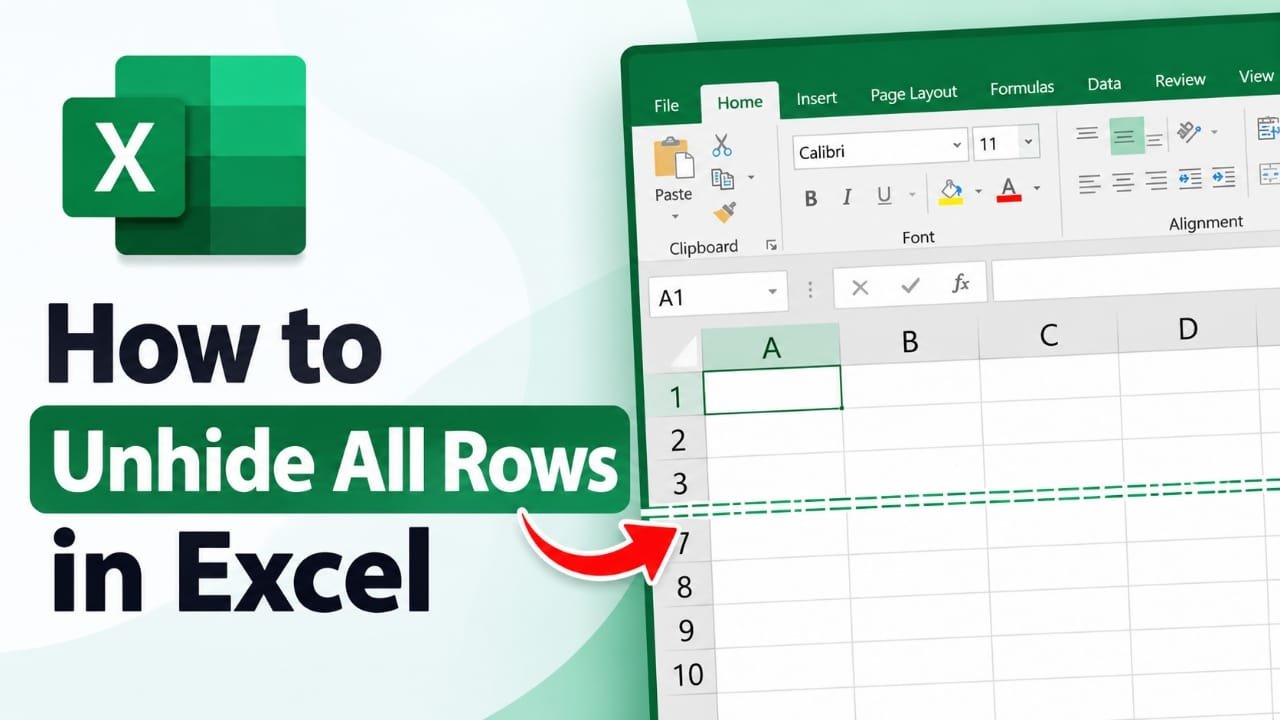
If some rows are missing from an Excel worksheet, they may simply be hidden. You can usually bring them back in a few clicks without changing the data in those rows.
The easiest method is to select the entire worksheet and use Unhide Rows. This guide explains how to unhide all rows in Excel on Windows, Mac, and the web, along with solutions for rows that still appear to be missing.
Also read: How to Back Up an Android Phone Without Losing Your Important Data
How to Unhide All Rows in Excel
If you want every hidden row in the worksheet to become visible, select the entire sheet before using the Unhide command.
On Windows
- Open the Excel worksheet.
- Click the Select All button in the top-left corner, where the row and column headings meet.
- You can also press Ctrl+A to select the worksheet.
- Right-click any row number on the left side.
- Select Unhide.
Excel will show the hidden rows covered by your selection.
If pressing Ctrl+A selects only the current data area, press it again to select the entire worksheet.
Using the Home tab
You can also unhide rows through the Excel ribbon:
- Select the entire worksheet.
- Open the Home tab.
- Click Format in the Cells section.
- Select Hide & Unhide.
- Click Unhide Rows.
On Windows, you can also use the ribbon keyboard sequence Alt, H, O, U, R, pressing each key separately.
How to Unhide All Rows in Excel for Mac
The process is similar on a Mac.
- Click the Select All button in the top-left corner of the worksheet.
- Alternatively, press Command+A.
- Right-click or Control-click a row number.
- Choose Unhide.
You can also use the menu:
Home → Format → Hide & Unhide → Unhide Rows
If you are using a trackpad, a two-finger click can be used to open the context menu.
How to Unhide Rows in Excel for the Web
If you are working with Excel in a browser:
- Open the workbook in editing mode.
- Select the entire worksheet using the triangle in the top-left corner.
- Right-click a row number.
- Select Unhide Rows.
If the option does not appear, make sure you clicked a row number rather than a cell.
Also check that the workbook is not open in view-only mode. You need editing access to change row visibility.
Excel Keyboard Shortcuts for Unhiding Rows
Keyboard shortcuts can make the process faster.
| Excel version | Select the worksheet | Unhide rows |
|---|---|---|
| Windows | Ctrl+A | Ctrl+Shift+9 |
| Mac | Command+A | Shift+Command+( |
| Excel for the web | Ctrl+A | Ctrl+Shift+9 |
On the web version, your browser may sometimes intercept a keyboard shortcut. If the shortcut does not work, use the right-click method instead.
How to Unhide Only Specific Rows
You do not always need to restore every hidden row.
Suppose the row numbers jump from 10 to 15. That usually means rows 11 through 14 are hidden.
To restore them:
- Select the row immediately above the hidden section.
- Select the row immediately below it.
- Right-click the selection.
- Choose Unhide.
You can also double-click the line separating the visible row numbers around the hidden area.
This method is useful when you want to keep other rows hidden.
How to Unhide Row 1 in Excel
The first row can be slightly different because there is no visible row above it to select.
If row 1 is hidden:
- Click the Name Box beside the formula bar.
- Type
A1. - Press Enter.
- Open Home → Format → Hide & Unhide.
- Select Unhide Rows.
Another simple option is to right-click the row 2 heading and choose Unhide Rows.
If multiple rows at the top are hidden, selecting the entire worksheet and using Unhide Rows is usually easier.
How to Check Whether All Rows Are Visible
After unhiding the rows, look at the row numbers on the left.
A normal worksheet should show consecutive row numbers without unexplained gaps. If the numbering still jumps, something other than standard row hiding may be preventing the rows from appearing.
You can also scroll toward the top of the worksheet and check whether row 1 is visible.
If you accidentally unhide rows and want to reverse the change, use:
- Ctrl+Z on Windows or Excel for the web
- Command+Z on Mac
Why Excel Rows May Still Be Missing
Sometimes clicking Unhide does not solve the problem because the rows are not hidden in the normal way.
Check these possibilities.
1. A filter is hiding the rows
Filtered rows are different from manually hidden rows. The Unhide command does not remove a filter.
To clear the filter:
- Open the Data tab.
- Select Clear.
If you want to remove filtering completely, use the Filter option on the Data tab.
A filter may be active if the worksheet shows filtered row numbers or filter controls in the column headings.
2. The worksheet is protected
Protection can prevent you from changing row visibility.
Go to:
Review → Unprotect Sheet
If Excel asks for a password, you will need the password that was used to protect the worksheet.
If you do not have it, contact the person who created or protected the workbook rather than trying to bypass the protection.
3. Rows are grouped
Excel can group rows into an outline. When a group is collapsed, some rows disappear from view.
Look along the left side of the worksheet for plus (+) or minus (-) buttons.
Click a plus button to expand a collapsed group.
If you want to remove the grouping, you can use the options under:
Data → Ungroup
Be careful when changing outlines because collapsed groups can make rows appear missing even though the underlying data is still there.
4. The row height is extremely small
A row can sometimes have a very small height instead of being normally hidden.
Select the affected rows and go to:
Home → Format → Row Height
Enter an appropriate value and select OK.
You can also use AutoFit Row Height when you want Excel to adjust the row based on its contents.
Be careful when applying a single height to the entire worksheet because it can replace custom row sizes.
5. Freeze Panes are making rows difficult to reach
Frozen panes can sometimes make it look as though rows are unavailable, especially when you are working with a large worksheet.
To remove the frozen panes:
View → Unfreeze Panes
Then scroll through the worksheet again and check whether the missing rows are actually there.
What If Only Some Rows Come Back?
This usually means your original selection did not cover the entire worksheet.
Click the Select All button and run Unhide Rows again.
Remember that Excel applies the Unhide command to the selected area. If you selected only part of the worksheet, rows hidden outside that selection may remain hidden.
Does Unhiding Rows Delete or Change Data?
No. Unhiding a row simply changes its visibility.
The information in the row remains in the worksheet. Unhiding it does not, by itself, delete the row, modify its values, or remove its formulas.
For example, if a worksheet contains a hidden row with sales data, unhiding the row makes that information visible again.
How to Unhide Rows and Columns Together
Rows and columns have separate visibility commands.
To restore both:
- Select the entire worksheet.
- Right-click a row number and select Unhide.
- Right-click a column letter and select Unhide.
You may need to perform the two operations separately.
What If Rows Hide Again Automatically?
If rows disappear again after you restore them, check for:
- An active filter
- Collapsed row groups
- Worksheet or workbook automation
- Macros that change row visibility
Clear the filters and expand any grouped rows first.
If the rows continue disappearing, the workbook may contain a macro or other automation that is changing their visibility. In that situation, the person who created or manages the workbook may need to check its settings or code.
Frequently Asked Questions
What is the shortcut to unhide all rows in Excel?
First select the worksheet with Ctrl+A, then press Ctrl+Shift+9 on Windows. On Mac, use Command+A, followed by **Shift+Command+(`.
Why is the Unhide option disabled in Excel?
Worksheet protection is one common reason. Check the Review tab for Unprotect Sheet. If the sheet requires a password, you need the correct password to remove the protection.
Can I unhide the first row in Excel?
Yes. You can select cell A1 through the Name Box and then use Home → Format → Hide & Unhide → Unhide Rows. You can also right-click row 2 and select Unhide Rows.
How do I unhide columns in Excel?
Select the columns around the hidden area, right-click the column letters, and select Unhide. You can also select the whole worksheet and use the column Unhide command.
Will unhiding rows affect formulas?
Unhiding rows does not itself change formulas. It only makes previously hidden rows visible.
Why are rows still missing after I click Unhide?
Check whether a filter is active, the rows are grouped, the worksheet is protected, the row height is extremely small, or panes are frozen. These situations can make rows appear missing without normal row hiding being the cause.
Can I undo unhiding rows?
Yes. Use Ctrl+Z on Windows or Excel for the web, or Command+Z on Mac.
Also read: How to Factory Reset an Android Phone Safely
Final Takeaway
For most Excel worksheets, the quickest solution is simple: select the entire worksheet, right-click a row number, and choose Unhide.
If that does not restore the missing rows, do not keep repeating the same command. Check filters, worksheet protection, grouped rows, row height, and frozen panes. One of these is often responsible for rows that appear to be missing.
Before printing, sharing, or reviewing an important workbook, it is also a good idea to check whether filters or hidden rows are intentionally hiding information.

Abhi Rajput, founder of Earnabhi.com, is a tech lover with 6+ years of experience in SEO, digital tools, and smartphone troubleshooting. He writes simple, clear, and useful guides to help people solve real tech problems.